General Derivation: Directional at the 3rd Moment (N = 3)
We've examined the algebra of the Directional's 1st two moments. The 1st moment of both the Living Average and the Directional are identical, the value of the 1st data byte divided by the Decay Factor (X1/D). The 2nd moment only differs by one factor. Let's see what happens when we apply the same analysis to the 3rd moment. What will our search for a data-based equation reveal?
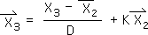
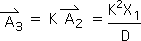
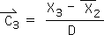
3.1 Let's begin with the Living Algorithm's context-based equation for the Directional at the 3rd moment (N = 3).
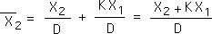
3.2 We already know the Living Average at the 2nd moment (Equation 2.9).
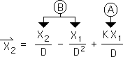
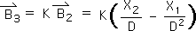
3.3 We also know the Directional at the 2nd moment (Equation 2.24). It is shown below with components for future reference.
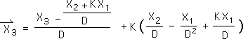
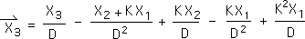
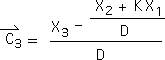
3.4 We plug these data-based equations into Equation 3.1 with the following result.
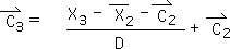
3.5 We perform a slight algebraic simplification. This is the data-based equation for the Directional at the 3rd moment.
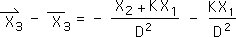
3.6 A bit of a mess. Let's compare it with the Living Average at the 3rd moment. We show it with the horizontal components identified (Eq. 23).
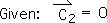
3.7 Notice how for the 3rd moment (N = 3) that the Directional (Eq. 3.5) contains all the positive elements of the Living Average (Eq. 3.6). A simple subtraction of the two equations yields the following difference. Only the negative components remain. It is evident that when the data is positive that for the 3rd moment that the Directional is the same as the Living Average - just a little less.
Besides being a mess, the data-based expression for the Directional at the 3rd moment (Eq. 3.5) does not reveal the size of the info quanta (the colored rectangles of the Directional Grid).
Event-based Derivation: Directional at the 3rd Moment (N = 3)
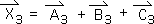
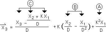
3.8 Let's analyze the Directional at the 3rd moment from an Event-based perspective to see what they reveal about our info quanta. As per our previous analysis, the individual contributions of the 3 Events (A, B, & C) at the third moment (N = 3) provides the total value of the Directional.
3.9 Let's start with Event A's contribution. As always, we merely scale the previous influence to obtain the current influence. This process always holds true. We scale (multiply by K) the value of the previous influence (Eq. 2.17) to obtain the data based equation we are looking for.
3.10 We apply the same analysis to uncover Event B's contribution to the 3rd moment. We scale the previous influence (Equation 2.20) to find the current influence.
3.11 By definition the 3rd data bit's entry into the Living Algorithm System initiates Event C. Employing the general Directional Equation (Eq. 2.1) determines the initial impact of Event C upon the Directional Grid.
3.12 Because this is the initial impact of Event C upon the System there are no prior Directionals by definition.
3.13 Two terms drop out leaving us with this context-based equation – just one composite term left.
3.14 Equation 2.24 reveals the value of this composite term (the Living Average of the 2nd moment). We plug it into the above equation to get the desired result – a data-based equation for the initial impact of Event C upon the total Directional at the 3rd moment.
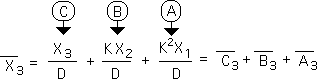
3.15 We plug the influences of Events A, B and C into the Event sum Equation 3.8. The following data-based equation is the result – complete with the components identified. Cross checking: this result is the same as Equation 3.4, which we came across from a different route.
Living Average Quanta function of Event’s Data Byte;
Directional Quanta function of Data Stream
3.16 A quick comparison of the Directional and Living Average at the 3rd moment is revealing (Equations 3.15 and 3.16). In the Living Average Grid, Events A, B, and C are functions of the data that spawned them. For instance, Event A is a function of the first data byte, X1. Similarly Event B is a function of the 2nd data byte, X2. The Directional Grid is quite a contrast. In this case, each Event A, B, and C are functions of all the preceding data. For instance, Event B is a function of both X1 and X2, while Event C is function of X1, X2, and X3.
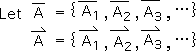
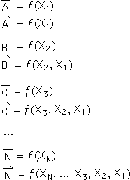
3.17 Let us remember our notation for Events. 'A bar' equals the data stream consisting of all the values in Living Average Event A. And 'A arrow' equals the data stream consisting of all the values in Directional Event A.
3.18 Each Living Average quantum is a function of the Data that spawned the Event. Each Directional quantum is a function of all the preceding Data. The Directional process certainly provides a layer of interactional complexity, not found in the Living Average process.
Living Average Grid: Data Byte only influences Info Quanta in its Event
Reiterating for emphasis: in the Living Average Grid, the value of each quantum of info energy (the color rectangles) is a function of a single data byte. This is because each data byte's individual influence is isolated to its Event. Each Living Average Event has one and only one data byte associated with it. As such, each Living Average Event is completely isolated from every other Event. In the Living Average Grid, the impact of each data byte has nothing to do with the other data bytes. The influence of each data byte is isolated to its Living Average Event.
Directional Grid: Data Bytes influence all subsequent Quanta of Info Force
In contrast, each data byte interacts with the earlier data bytes in intriguing ways to generate the Grids of the higher data stream derivatives – the Directional (the Active Pulse) and Liminals. This interaction is why the higher measures behave in such an unusual fashion. More specifically, each quantum of info force in the Directional Grid is a function of all the preceding data bytes, not just a single data byte. After entering the System, each piece of data in the stream exerts an influence on every quantum of info force that follows, not just the quantum in its Event. This influence depends upon proximity to the rest.
Living Average: Data Impact upon Event. Directional: Data Impact upon the Grid
Summarizing: In the Living Average Grid, data bytes only exert an influence upon the Event that they spawns. In the Directional Grid the data bytes exert an influence upon entire Grid.
Living Average vs. Directionals: Impacts differ; Influences the same
Data Stream Location: Directional Events crucial – Living Average Events unimportant
Let's explore some other implications of this intriguing finding. Because of the isolation of Events and their data, the values of the Living Average Events have nothing to do with where they enter the stream. In other words, location in the data stream has no effect upon the values of the Living Average Event streams. In contrast, the relative position in the data stream has everything to do with the values of the Directional Event stream. Location, location, location.
The Past a Factor in determining the Initial Impact of Data Bytes in Directional Grid – not so with Living Average Grid
The reason that data stream location is so important in the Directional Grid has to do with the Initial Impact of the data byte on the System. In the Living Average Grid, the Initial Impact of the data byte is identical, no matter where and when it enters the System. In the Directional Grid, the Initial Impact of the entering data byte is determined by what went before. The same data byte might exert a big Impact at one point in the stream and a smaller Impact at another point.
Current Influence in both Grids determined by Scaling Prior Influence or Impact
However, after the data byte's Initial Impact upon the Grid, the treatment of subsequent Influences in either Grid is identical. In other words, to determine the next value in any Event stream, whether Living Average or Directional, scale the previous Influence to determine the current Influence. In other words, multiply the past Influence (or Impact) by K, the Scaling Factor, to determine the current Influence.
Initial Impact is only difference between Living Average and Directional Grids
Therefore, the entire difference between the determination of the quantum values in the Living Average Events and Directional Events has to do with the Event’s initial Impact. After the initial Impact, the subsequent Influences in both Grids are determined in an identical fashion. The Past (the Influences of prior data bytes) is a factor in determining the value of the Directional Impacts, while Living Average Impacts are independent of the Past. Directional Impacts are influenced by all prior data bytes, while Living Average Impacts are independent of prior data bytes. However once the data byte has made its Impact on either System the values of the subsequent Influences in both Grids are determined in identical fashion, a simple scaling. There are no more external influences to take into account. There is no recovering or adjustment after the initial Impact. The interactive feedback between the data bytes based upon data stream location creates the interesting dynamics that result in the Active Pulse, a.k.a. the Pulse of Attention.
To see what our mathematical findings reveal about the intriguing behavior of our friend, the Active Pulse, check out the next article in the stream – Info Quanta in the Active Pulse.